
Guides / illustrated walkthrough
CLM-8B: the Contrastive Decision Model That Scores 1,024 Options in 44 ms (13x Faster Than Jev)
The Prompt Engineering deep-dive on CLM-8B (CLM-v0.1), turned into a step-by-step architecture walkthrough: the CLIP-for-decisions two-tower design, cached action embeddings that keep 1,024 options at 44 ms (Jev: 570 ms), the three-stage contrastive training recipe on a frozen Qwen3-8B, the DGX Spark demo stack, the 1,080-tool router and WikiRace replays — with the 86%-to-17% accuracy drop kept in.
Quick takeaway
This is an architecture deep-dive on CLM-8B (CLM-v0.1), a Contrastive Language Model from a Stanford + NVIDIA Research team claiming up to 9x faster decisions than Jev at on-par accuracy — not by shrinking the model, but by turning decision-making into retrieval. A frozen Qwen3-8B backbone ("just a reader") encodes the state; two ~20M-parameter heads embed state and actions into one space, so scoring 1,024 options costs one state embedding plus dot products: 44 ms on the video chart where Jev sits at 570 ms and a generic constrained-decoding LM climbs to 4,185 ms — about 13x — and the CLM line barely bends as candidates grow. It speaks Jev's three primitives (yes/no, multi-choice, score) over a closed candidate list: it can never invent an off-list answer, but it can confidently pick a wrong on-list one. Training is three ordered stages — 60M NVIDIA Nemotron QA pairs, then 30M Gemini-generated hard negatives (52% to 69% on a hard-negative test when the hard-negative stage comes after; mixed in from day one it stalls at 62% and overfits), then ~1M real agent-trajectory steps with 40% QA replay (without the replay, hard-negative scores fall 69 to 56). Because the backbone never changes, the dataset is embedded once and a full pre-training run takes about one hour on a single RTX 4090. On a DGX Spark (GB10), the whole stack — a vLLM-served Qwen3-8B encoder plus the team's ~75 MB CLM server, ~25 GB of memory — scores a support ticket (charged twice, cannot reach anyone) at urgent 84%, billing 99%, frustration "very angry", and re-scores the cached ticket in under 2 ms (0.8 ms model latency, 9 ms round trip, zero tokens re-encoded). The honest part: top-1 accuracy fell from 86% (77/90) with 8 tools to 17% (5/30) with all 1,080 — the state encoder never compares options side by side, so look-alike "refund" tools blur together — and the rebuilt WikiRace agent reached its target in 4 clicks in just one of the five races shown. The recommended pattern: let CLM cut 1,000 candidates to a top 10 in milliseconds, then let a model that reads options side by side (System 2) make the final call; small, stable action sets work directly. As of the video (2026-09-26) CLM is text-only; a 35B multimodal version was promised for the following month.
Video source
Prompt Engineering
Step-by-step walkthrough
- 1
What is CLM-8B? Stanford and NVIDIA contrastive language model
Jev made System 1 models hot again — small, non-reasoning models that answer "which tool next? is this ticket urgent? which link should the agent click?" in milliseconds. Most open replications, though, are still language models under the hood: they read your text, read every single option, and decode an answer token by token. CLM-v0.1 — a Contrastive Language Model from a Stanford + NVIDIA Research team — landed with a different architecture. It is an 8-billion-parameter model, the same size class as those clones, and the team claims up to 9x faster than Jev at on-par accuracy. The important part: the speed does not come from making the model smaller. It comes from how the thing is built, which is what the rest of this page unpacks — plus a working demo on a single DGX Spark. Note the framing on the card itself: the LLM decoder is crossed out entirely.
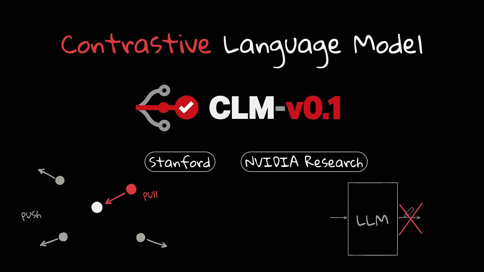
CLM = contrastive language model — the LLM decoder is crossed out of the design entirely.Watch at 1:01 - 2
CLIP, but for decisions: the two-tower architecture
The mental model the video offers: CLIP, but for decisions. CLIP put images and text into one embedding space, so a photo of a dog lands next to the words "a photo of a dog". CLM does the same with situations and actions. A state encoder reads what is happening right now; an action encoder reads what you could do. Take Mario with a Goomba walking toward him: the state is the game screen, the actions are left, jump, or run right. To decide, you embed the state once, embed every option, and score each option by how close it lands to the state in that shared space. A softmax over those scores turns closeness into probabilities — in the video example jump gets 80%, run right 15%, left 5% — and Mario jumps. No token is ever generated; the answer was decided by geometry.
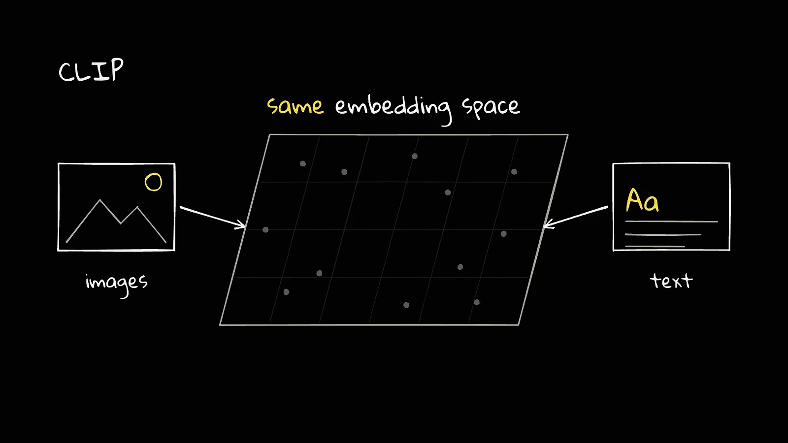
CLIP aligned images with captions; CLM aligns situations with actions in the same kind of shared space.Watch at 2:00 - 3
It speaks the Jev API — with the same fine print
CLM was designed to speak the same Jev API, so it exposes the three typed primitives this site keeps covering: a yes/no question, a multi-choice question, and a score. Underneath, all three are the exact same operation — a state plus a closed list of candidates; yes/no is just two candidates, true and false. That brings the same promise Jev made famous, and the same honest asterisk. It can never invent an answer that is not on the list — the "Jev can never hallucinate" line — but it can still pick the wrong answer from that list, and when it does, it can do so confidently. A fenced list stops invention; it does not stop a wrong pick from inside the fence. Keep that asterisk in mind — it comes back with numbers at the end of this page.
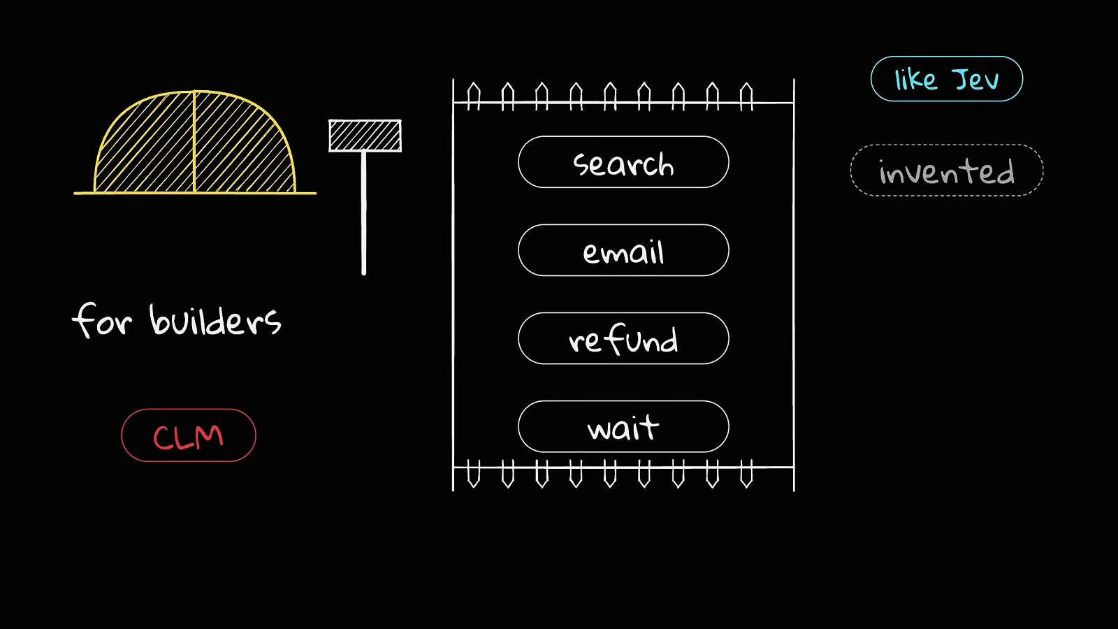
A fenced list the model cannot escape — but a fenced wrong answer is still wrong.Watch at 3:21 - 4
Where the speed comes from: embed the actions once, cache them
A Jev-style model puts the state and all the options into the model together on every call: double the options and you read twice as much, then decode the answer token by token out of a large model — expensive, and it compounds. CLM splits the two towers apart. In most agent loops the actions do not change from step to step; the state does. So you embed the actions once and cache them, and each new step costs one state embedding plus a dot product per option — and a dot product is essentially free computation. In the Mario demo that takes each step from five forward passes down to one. The frame shows the shape of it: the state encoder runs per step (that agent loop is at step 6 and counting), while the action encoder runs once for left, jump, run right, duck.
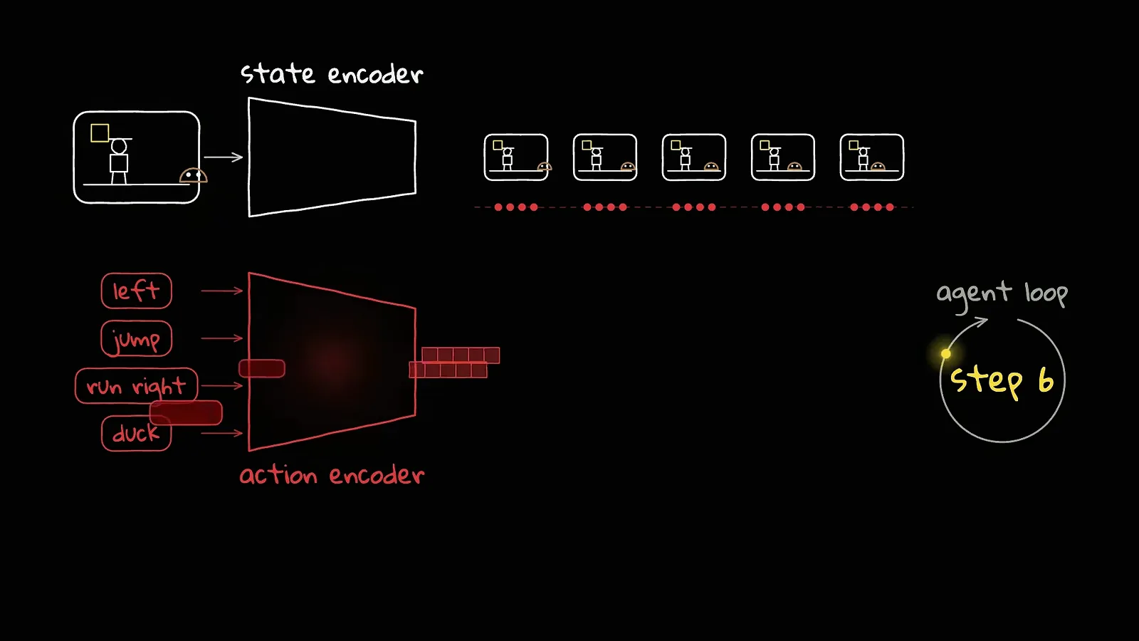
The state is encoded every step; the actions were embedded once and just get reused.Watch at 5:41 - 5
The 13x chart: 1,024 options at 44 ms vs Jev at 570 ms
This is the claim in the video title, on the team chart. As the candidate count grows from 1 to 1,024, the constrained-decoding line for a plain LM climbs to 4,185 ms; Jev sits at 570 ms at the right edge; CLM barely moves at all, landing at 44 ms. That is about 13x faster than Jev with a thousand options in the list — and the video earlier notes constrained decoding was already past four seconds by a few hundred options, which is exactly the regime real tool lists live in. In the System 1 / System 2 framing from an earlier video, System 1 scales in width — lots of small questions answered at once — and CLM pushes that about as far as it will go: a thousand options for roughly the price of one.
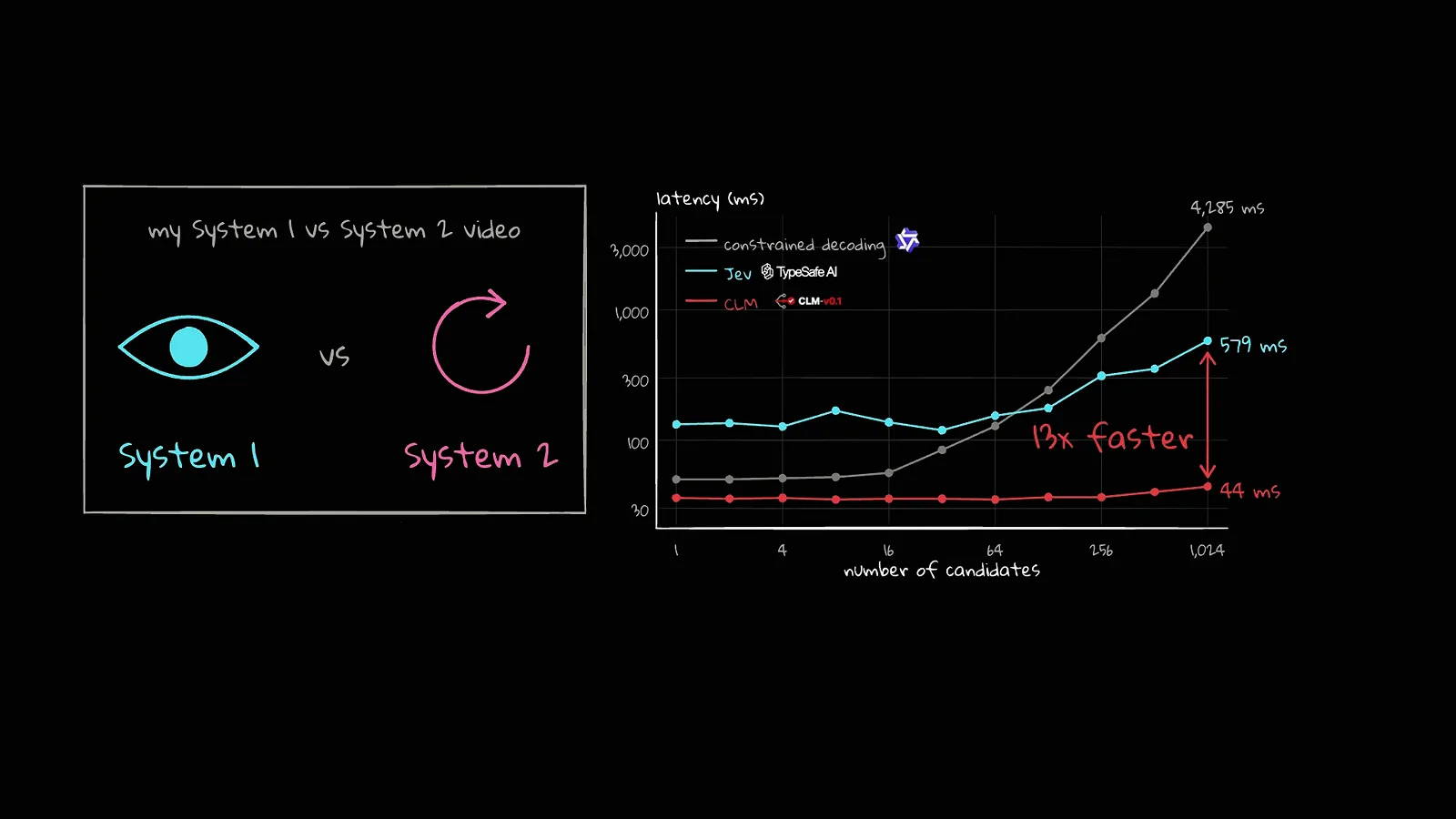
Candidate count barely moves the CLM line: 44 ms where Jev needs 570 ms at 1,024 options.Watch at 6:25 - 6
The catch: the state never sees the options
Here is the classic trade-off of every two-encoder design, and the video does not hide it. Because the state is encoded on its own, it never sees the options. It cannot lay them side by side and compare them; every candidate is judged alone, in isolation, against a situation vector it cannot revisit. When the options are meaningfully different — jump versus run right — that is fine. When options blur together — three refund tools with different names and nearly identical descriptions — judging each alone is exactly the wrong way to compare them. This one architectural property is the root cause of the accuracy collapse you will see in the 1,080-tool experiment below, so hold onto it: the same design that makes scoring cheap makes comparison impossible.
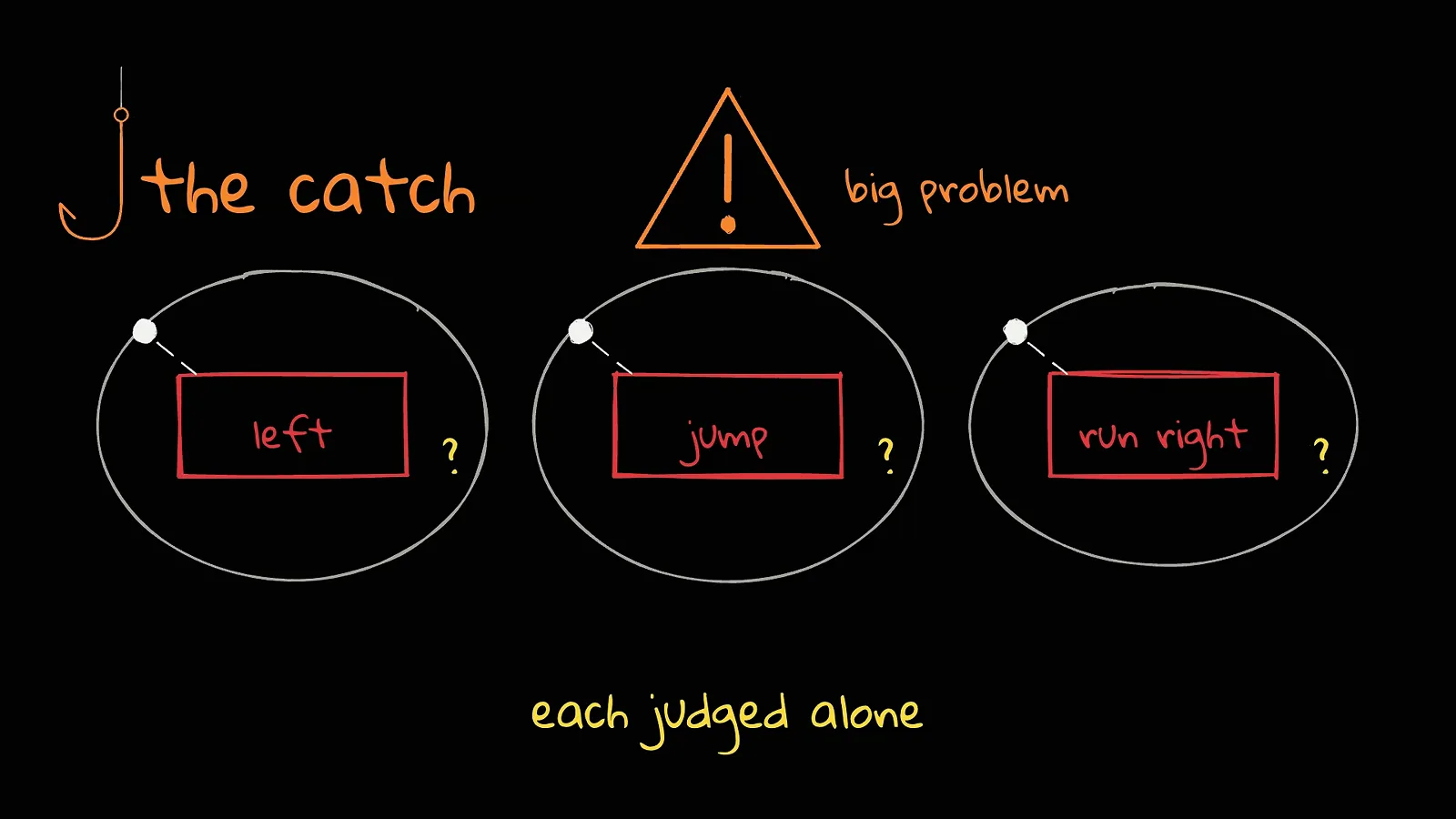
Each option judged alone — no side-by-side comparison, ever. Remember this chart for step 13.Watch at 7:01 - 7
Three training stages — and why the order matters
Why not just use any embedding model? Because similar is not the same as right: ask raw Qwen3-8B embeddings who wrote Romeo and Juliet and Shakespeare does not come first — in the video demo Christopher Marlowe ranks #1 at 23.9% with Shakespeare second at 22.2% (the theory slide had him even lower, third). CLM gets to "right" by contrastive training in three stages. Stage 1: 60 million question-answer pairs from NVIDIA Nemotron data — question is the state, answer is the action — to learn world knowledge. Stage 2: 30 million Gemini-generated hard negatives, answers that are close but wrong (Venus instead of Mercury for the planet closest to the sun), which teach the difference between sounds right and is right. The order is load-bearing: on a hard-negative test, pre-training alone scores 52%, adding the hard-negative stage on top jumps to 69% — but mixing hard negatives in from day one peaks at 62% and then overfits. Stage 3 turns it into an agent: about a million steps of real agent trajectories, mixed with 40% of the original QA data replayed back in; without that replay, hard-negative scores fall from 69 to 56.
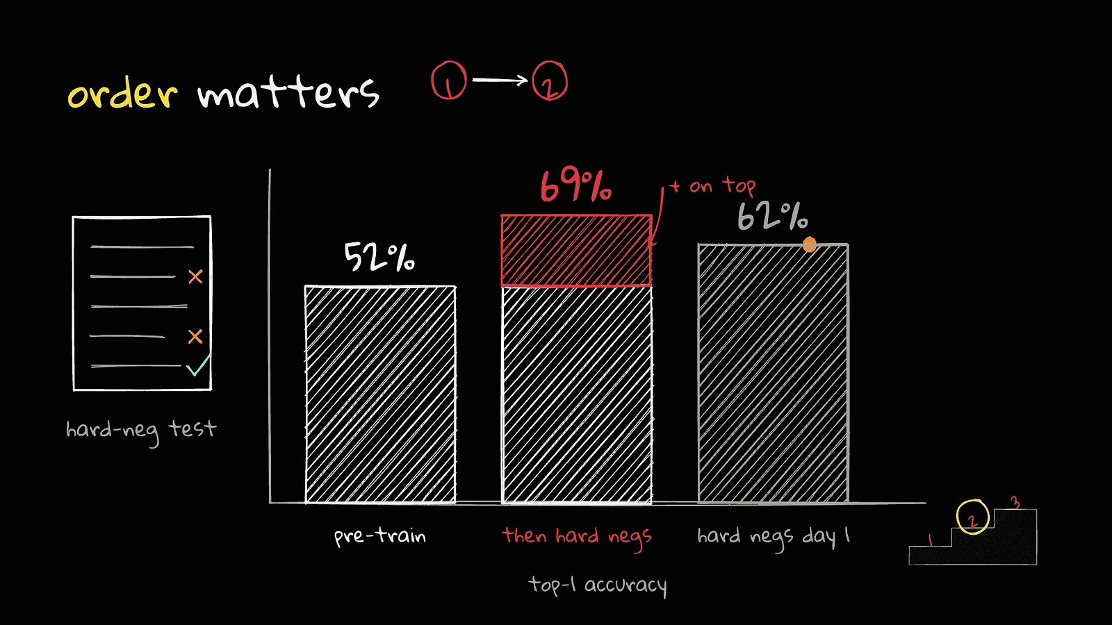
Learn the world first, fine distinctions second: 52 to 69% — but 62% and overfitting if you flip the order.Watch at 8:27 - 8
The backbone is frozen: only ~40M parameters ever train
The part that surprised the video creator: the 8-billion-parameter model is frozen. The backbone is Qwen3-8B used as a reader — it receives a single gradient, the card literally labels it "just a reader" with a padlock. The only things that train are two small heads, about 20 million parameters on each side of the tower. Because the backbone never changes, you embed the whole dataset once, and after that a full pre-training run takes about one hour on a single RTX 4090 — for an 8B-class model, which is close to absurd. The loss follows a power law (the chart shows a -0.172 exponent in encoder size) across compute, data, head size, and encoder size, and encoder size gives the biggest gains of the four — which is exactly why the team says a bigger backbone is next. One timeliness note: as of this video (2026-09-26) the released model is text-only, and the 35B multimodal version was promised for "early next month" — check the official repo before quoting any of that.
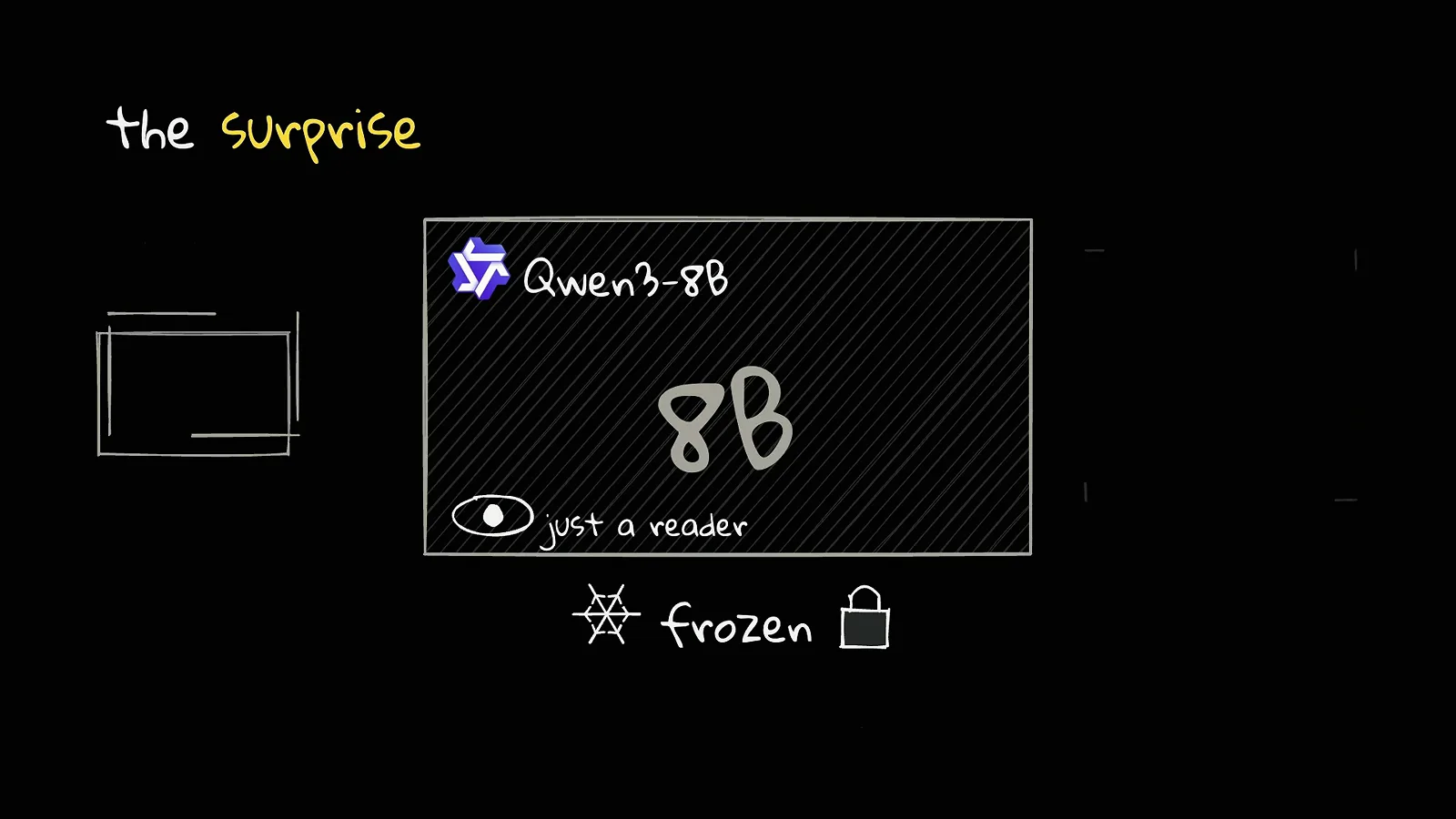
The 8B reader never updates — only the two ~20M-parameter heads train, so pre-training reruns in about an hour on a 4090.Watch at 9:21 - 9
Hands-on: the whole stack on one DGX Spark
All the demos in the second half run on a single DGX Spark (the GB10 box). The layer cake: the Qwen3-8B encoder served through vLLM — the terminal shows the vllm/vllm-openai container up 26 hours — with the CLM server the team actually released sitting on top. The server itself is about 75 MB; the whole thing takes about 25 GB of memory. The first demo feeds it a support ticket — a customer charged twice who cannot reach anyone — and asks three typed questions in one call: Is this urgent? Which team should handle it? How frustrated is the customer? Every answer comes back as a probability: urgent 84% (83.7% on the readout), billing 99%, frustration "very angry". And once the ticket has been seen, asking again returns in under 2 ms — the model latency reads 0.8 ms, round trip 9 ms, encoder_tokens 0 — because nothing gets re-encoded; the option vectors are all cached.
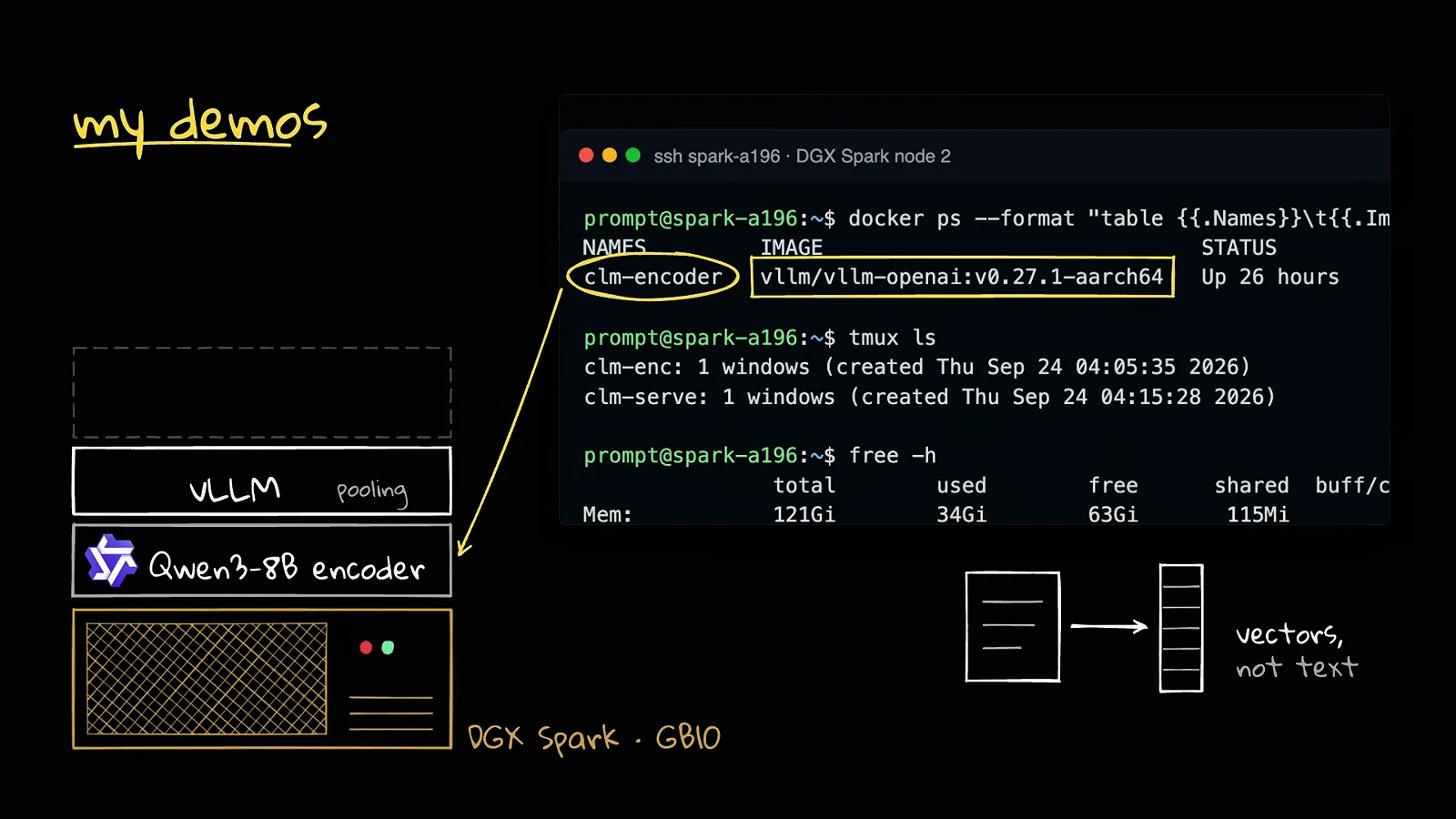
vLLM serves the frozen encoder; the ~75 MB CLM server on top turns vectors, not text, into decisions.Watch at 10:10 - 10
Watch the head move Shakespeare from 22% to 98.2%
The Romeo and Juliet question comes back as a live A/B test of the architecture: same encoder, same candidates — the only difference is the small head on top. With raw Qwen3-8B embeddings, Christopher Marlowe comes first at 23.9% and William Shakespeare second at 22.2% — reasonable-sounding companies for the authorship, wrong answer. Switch to the trained CLM head and Shakespeare jumps to 98.2%, first place. That is what ~20 million trained parameters do: they reshape the embedding space from similar to right, which is exactly what the hard-negative stages in step 7 paid for. It is also the cleanest one-frame demonstration of why "we already have embedding models" is not a counterargument to this architecture — plain retrieval finds similar things; a contrastively trained decision head finds the right one.
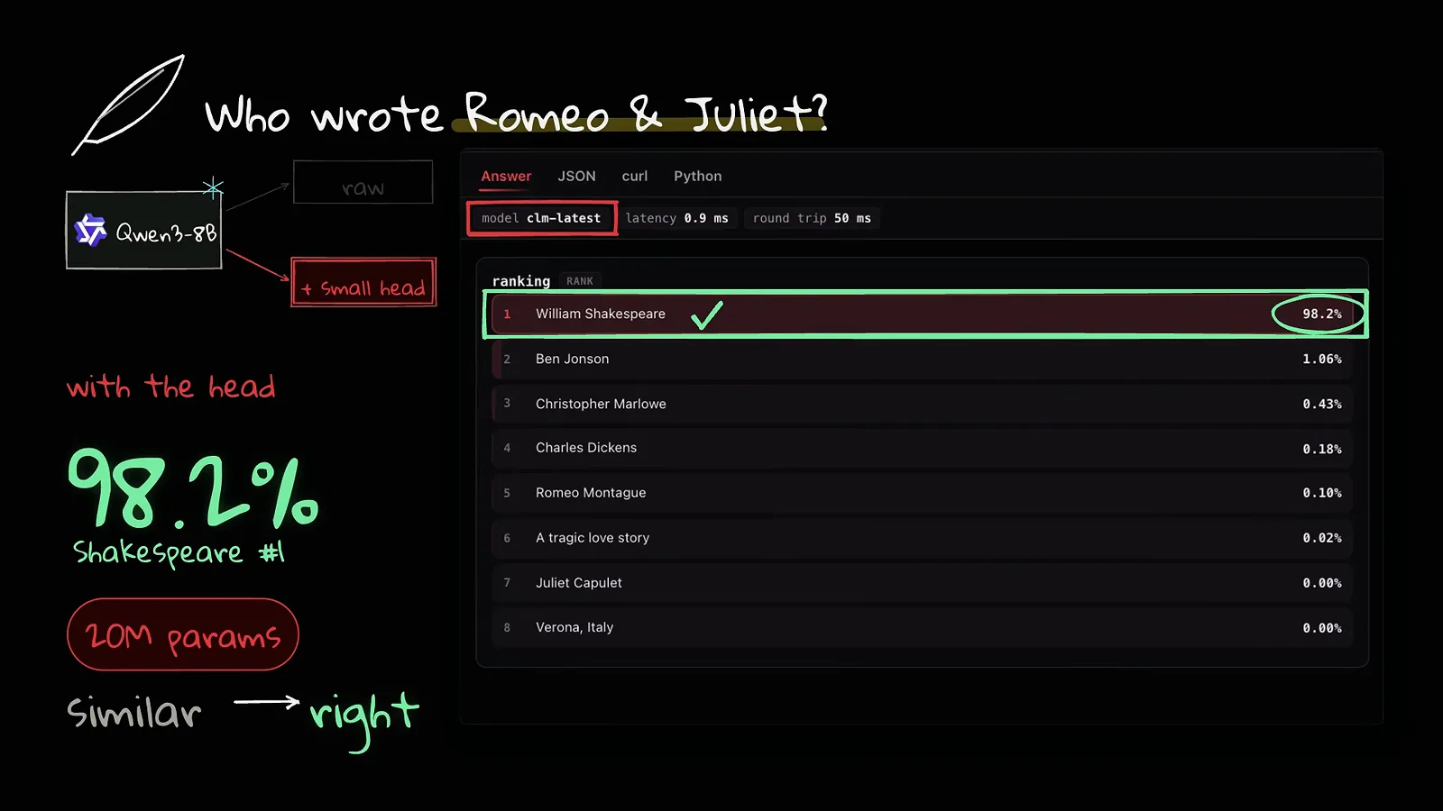
Same encoder, same candidates — 20M trained parameters turn "similar" into "right" (98.2% Shakespeare).Watch at 11:37 - 11
Routing 1,080 tools — a list Jev cannot even fit in one call
Now the architecture shows off. The creator built a list of 1,080 tools — Stripe, Twilio, QuickBooks, Zoom and so on — to route requests against. Two things matter here. First, Jev literally cannot take this list: a Jev choice call caps at 255 options, so 1,080 will not fit into a single call no matter how you slice it. Second, CLM eats it: the first request takes a few seconds (6,788 ms on screen) because the model embeds every tool once, and after that every new request takes about 80 milliseconds — the per-request lines on screen read 79 to 84 ms. The video also shows a timing table where, once cached, picking from 1 tool or from 1,024 costs basically the same: 0.5 ms versus 2.9 ms in the hot column. Embed once, then the option count is a rounding error on your latency bill.
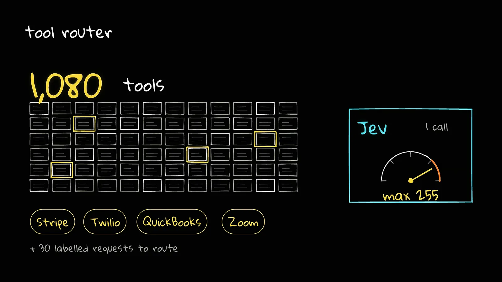
1,080 tools in one list — over Jev's 255-option cap, and just one embedding pass for CLM.Watch at 11:53 - 12
WikiRace replay: 934 links scored in one pass, reached in 4 clicks
The fun one. The WikiRace demo code was never released, so the creator rebuilt it himself: start on one Wikipedia page, reach a target page by clicking links. From Plate tectonics to Bioluminescence, CLM scores every single link on the page toward the target — 934 links ranked in 84 ms on the first screen, with Biosphere on top at 27.2%, Abiogenesis at 16.7%, Biogeochemical cycle at 13.0%. The strategy is greedy with no lookahead (max 15 clicks): pick the top-scored link, rescan, repeat. That took 4 clicks — Plate tectonics → Biosphere → Biota (ecology) → Plankton → Bioluminescence — versus about 6 in the team own demo. Read the card honestly, though: of the five races shown in that header row, only this one succeeded — Chess to Volcano, Jazz to Photosynthesis, Pizza to Albert Einstein and Tokyo to Penguin all failed. Some races it nails; others it wanders, for the same two-tower reason as the next step.
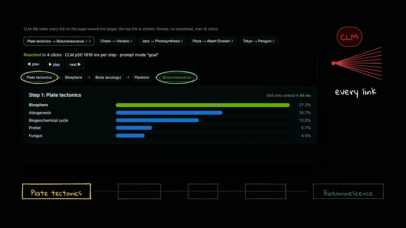
Every link scored at once — 934 in 84 ms — and a greedy clicker that reached the target in 4 hops (1 of 5 shown races).Watch at 12:41 - 13
The honest numbers: 86% at 8 tools, 17% at 1,080
What scales beautifully is compute; what does not is accuracy. With 8 tools to choose from, CLM picked the right one 86% of the time (77 of 90 top-1 in the creator run). With all 1,080 tools, that fell to 17% (5 of 30) — mostly because it confused tools that sound alike: refund (Stripe) versus refund (QuickBooks) versus refund (PayPal). The WikiRace card said the same thing — some races nailed, some wandered. This is the catch from step 6 showing up in measurements: each option is encoded on its own, so the model never compares them side by side, and look-alike options are indistinguishable at any speed. The video advice is the takeaway: do not hand an agent 1,000 tools — build sub-agents with smaller tool sets. The way to use CLM today is as a first stage: let it cut a thousand candidates to a top 10 in milliseconds, then let a model that reads options together — System 2 — make the final call. If your action set is already small and stable (a game loop, a handful of routes), it works well directly. And the standing caveat for every number on this page: these are the video creator runs on his own demos, not an independent benchmark.
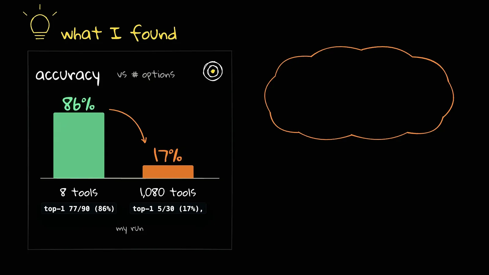
Latency scales; accuracy does not: 86% to 17% as the tool list grows 135x.Watch at 13:41
Frequently asked questions
What is CLM-8B?
CLM-8B (released as CLM-v0.1) is a Contrastive Language Model built by a Stanford + NVIDIA Research team: an 8-billion-parameter model whose Qwen3-8B backbone is frozen and used purely as a reader, with two small trained heads (~20M parameters each) embedding states and candidate actions into one shared space. A decision is made by embedding the situation, embedding every option, and picking by distance — the video calls it "CLIP, but for decisions". The team claims up to 9x faster than Jev at on-par accuracy. Timeliness note: as of the video (2026-09-26) the released model is text-only, and the official repo name and the promised 35B multimodal follow-up should be re-checked against the project page before you quote them.
CLM-8B vs Jev — what is actually different?
The API shape is identical: yes/no, multi-choice, and score questions over a state plus a closed candidate list, with the same promise and the same fine print — it can never invent an off-list answer, but it can confidently pick a wrong on-list one. The engine underneath is completely different. A Jev-style model reads the state and every option together and decodes an answer with constrained decoding, so latency grows with the option list (570 ms at 1,024 options on the video chart; 4,185 ms for a generic constrained-decoding LM) and a single Jev choice call caps at 255 options. CLM-8B embeds the options once, caches them, and scores by dot products — 44 ms at 1,024 options, roughly 13x faster. The trade-off: Jev decoder sees all options side by side when answering; CLM judges each option in isolation, which is why its accuracy collapses on look-alike candidates.
Why is CLM faster than Jev?
Because it turns the decision into retrieval. Options are embedded once and cached; each new step costs one embedding of the state plus one dot product per option, and a dot product is essentially free computation. In agent loops the action list rarely changes, so the expensive part is paid once and amortized forever. On the video Mario demo this took each step from five forward passes down to one, and on the latency chart the candidate count going from 1 to 1,024 moves the CLM line from a few dozen milliseconds to 44 ms — while constrained decoding climbs to 4,185 ms and Jev reaches 570 ms. The option count becomes a rounding error instead of the dominant cost.
What does it take to run CLM-8B locally?
The video runs everything on one DGX Spark (GB10): the frozen Qwen3-8B encoder served through vLLM, with the CLM server the team released on top — the server itself is about 75 MB, and the whole stack takes roughly 25 GB of memory. Because option vectors are cached, re-asking about a seen state returns in under 2 ms (0.8 ms model latency, 9 ms round trip, zero tokens re-encoded). Training economics are equally mild: since the backbone never changes, you embed the dataset once and a full pre-training run takes about one hour on a single RTX 4090 — only the two ~20M-parameter heads ever update.
Does the 13x speed hold when the option list gets huge?
The latency does; the accuracy does not. Scoring 1,080 tools costs about the same as scoring one (the video table shows 0.5 ms vs 2.9 ms hot), but top-1 accuracy fell from 86% (77/90) with 8 tools to 17% (5/30) with all 1,080 — mostly confusion between sound-alike tools like three different "refund" endpoints. The cause is architectural: the state is encoded without ever seeing the options, so nothing is compared side by side. The video advice: do not give an agent 1,000 tools — split work across sub-agents with smaller tool sets, and use CLM as a millisecond first stage that cuts candidates to a top 10 before a System 2 model that reads options together makes the final call. Small, stable action sets (game loops, fixed routes) are where it works well as-is.
What is a contrastive decision model (contrastive language model)?
A model trained with a pull-and-push objective instead of next-token prediction: each training example is a situation plus an action somebody actually took, and the model learns to place the situation next to its own action and far from every other action. Negative examples come for free — the other 999 actions in a batch of 1,000 all belong to other situations — and the hard part is the 30 million Gemini-generated hard negatives, answers that are close but wrong (Venus vs Mercury), which teach the difference between "sounds right" and "is right". It is the same contrastive lineage as CPC/InfoNCE, SimCLR and CLIP, applied to decisions — which is why the video frames it as an old algorithm (hot in 2017-2018) making a comeback inside a System 1 model.
Related guides
Nox 4B: Testing the vLLM Decision 2.0 Family
A different fast-decision bet put through four scenario tests — this page is a single-model architecture deep-dive; that one is a hands-on family evaluation.
ReadClef-Flash: Install and Run It Locally
Another Jev-shaped decision model, covered as a from-zero Ubuntu install with a multimodal image demo — the installation axis, where this page is the architecture axis.
ReadJev Open Models: the Open-Weights Landscape
The 20-30 model reproduction panorama. Read it for breadth, then come here for the one architecture that breaks the LM-decoding mold.
ReadJev vs an LLM: System 1 Meets System 2
The concept page behind the "first stage vs final call" pattern that CLM-8B pushes to its limit.
ReadWhen to Use Jev (and When Not To)
The fit-boundary guide every decision model on this site inherits — including the 255-option choice cap that CLM-8B cached embeddings sidestep.
ReadBenchmarks: Our Own Measurement Standards
Every number on this page is the video creator run on his own demos; this is how we re-measure decision models ourselves before recommending one.
ReadMore video walkthroughs
- Jev Classification Quickstart: OpenRouter API, Primitives & Real Probabilities
- Jev Architecture Explained: Why 70ms Decision Models Beat LLMs for Workflow Automation
- Ultra-Fast Browser Agents with Jev: 178ms DOM Loops & Dual Model Orchestration
- Open Jev Models Are Here: Semif, Nimble, Decider, DiffusionGemma & Laya Hands-On
- Jev vs LLM: Will Jev Replace LLMs? Krish Naik's Whiteboard Explainer
- Jev Trader Tutorial: Build a Subsecond AI Trading Bot on Monad
- Jev Model Router: Build a Privacy-Gated LLM Router with Jev & OpenJev
- Jev Tutorial for Beginners: State, Questions & the TypeScript SDK
- Run Jev Locally: Kev, SemIf & Von on Your Own GPU (OpenJev Guide)
- Jev RAG Reranker: Policy-Steered Reranking for Retrieval-Augmented Generation
- When to Use Jev: An Engineer's Audit of Claims, Gates, and Failure Modes
- LangChain + Jev Integration Tutorial: Routing, Guardrails & Evals
- Jev MCP Server: Connect Jev Decisions to Claude Code & Cursor
- Jev vs Luna: Independent Benchmarks Put "Better, Faster, Cheaper" to the Test
- Jev Agent Harness: Where the Decision Gate Sits in Your LLM Loop
- Jev Playground Walkthrough: The Hotdog Lesson, Criteria, and a Four-Console Token Test
- Jev Text Classification API: Zero-Shot CLI & REST with classifier.dev
- Jev API Examples: First Request, curl & All Three Question Types
- Jev Log Triage with Expanso Edge
- Jev Lead Enrichment with Treg: ICP and Signup Scoring
- Use Jev Decision Nodes in Heym for Model Routing
- Laya Tutorial: Open-Source AI Routing With Calibrated Probabilities (Laya vs Jev Setup)
- Train Your Own Jev: Fine-Tune a Jev-Style Decision Model for $5–$17 (What You Can and Cannot Train)
- Jev Tips: 8 Best Practices for Better Decisions (State, Questions, Criteria & Thresholds)
- Jev Context Compaction: Prune AI Agent Memory Without Generative Summaries
- Jev as an LLM Judge: Confidence-Gated Cascades at 0.36% of the Cost
- TypeSafe Computer Use: Local Desktop Automation with Jev, Step by Step
- Jev Resume Screening: Build an AI Resume Evaluator with the Jev JavaScript SDK
- Jev + Claude Code Guide: Voice-Controlled Browser Automation with Typed Decisions
- Jev + Codex: Install the TypeSafe Skill and Triage a Real Gmail Inbox
- Jev vs Ollama: Can Local AI Replace Hosted Jev Without Sending Your Data Away?
- Build Your Own Jev: Train a Free Open-Source Zero-Shot Classifier (That Plays Doom)
- CUA-S1-Forms: a 706K-Parameter Jev-Like Model That Fills GUI Forms on Your CPU
- NOC/SOC Alert Triage with Jev: Rules First, One Typed Question, a Policy Gate
- Ollama Decision Models: Run tev1 and Nimble Locally (Tested on an 8 GB Card)
- Jev Guardrails in Production: A Five-Step Playbook for Decision Automation
- A Session Drift Guard for Pi Agent: Let the Jev Model Propose, Let Code Decide
- 50 Tev1 Use Cases: What a Local Decision Model Can Actually Do (Tested on an 8 GB Laptop)
- Jev, Hands-On: Where the Official Claims Meet Independent Remeasurement
- Jev Ticket Classification in a Real App: the After-Insert Hook and the Calculated Field
- OpenJev RLCD: Run the Open-Source Calibrated Decision Model Locally (Full Guide)
- Clef-Flash vs Jev: I Tested Cloudflare's Decision Model Locally in Ollama (Q4_K_M)
- Clef-Flash Tutorial: Install and Run Cloudflare's 9B Multimodal Decision Model Locally on Ubuntu
- Nox 4B Tutorial: Run the Decision 2.0 Model Locally and Put It Through Four Real Decisions (One Ends in a Fail)
- Julia-1 Tutorial: Install the Open-Source Jev Replacement in Pure Python (and Watch It Beat If-Statements 9 to 2)
- OpenJev 0.8B on CPU: I Built a Ticket-Routing Inbox and Calibrated the Thresholds
- Jev n8n Integration: the JevGate Community Node, Step by Step (Plus a Plain-HTTP Fallback)